Start
Research
Publications
Statistics playground
Teaching
CV
Contact
Stochastic processes play a vital role in describing many phenomena. In astrophysics in particular, recent years has seen a large increase in time-series data, e.g. from SDSS Stripe 82 or Kepler's asteroseismic observations. In many cases, these time-series data cannot be described by deterministic models but rather stochastic processes are required.
My personal interest in stochastic processes was allready sparked as an undergraduate, when I was fascinated to learn about the mathematics of Brownian motion. I picked up on this once I got interested in quasar variability and also in risk analysis of stock market values.
Stochastic processes in finance vs astrophysics
While stochastic processes are popular models in both, astrophysics and finance, there are a few fundamental differences: First, financial data is extremely well behaved in the sense that it comes (a) without any kind of measurement errors and (b) with regular time sampling. Conversely, astrophysical time-series data always has errors and irregular time sampling. A second important difference is that in astrophysics it is often sufficient to consider Gaussian processes (e.g. see my paper on QSO variability), whereas in finance the data exhibit decided evidence for non-Gaussianity (see Figure 1).
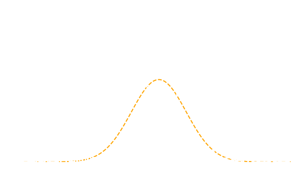 Figure 1. Distribution of daily log-returns of the MSCI World stock market index between 2007 and 2020 (white histogram) compared to a best-fit Gaussian (orange dashed line). The stock market data are more sharply peaked, have heavier tails and exhibit asymmetry.
This means that, in astrophysics, we are on the one hand "unlucky", having to cope with measurement errors. On the other hand, since our stochastic processes are usually Gaussian, it is easy to take Gaussian measurement errors into account. Moreover, for Gaussian processes, we can employ the powerful mathematical formalism of stochastic calculus (which has no equivalent for non-Gaussian processes).Fitting stochastic processes to data
Fitting time-series data with measurement errors using stochastic process models can be a challenge, both conceptually and computationally. It requires to convolve the model prediction of the stochastic process (which is a PDF) with the PDF of the measurement errors. Such a convolution may have no analytic results, which would make this computationally extremely expensive. Here, a Gaussian process with Gaussian measurement errors is a major advantage, since the convolution is fully analytic. As is evident from Figure 2, this must be taken into account when fitting the data, since the measurement errors do not contribute to driving the stochastic process.
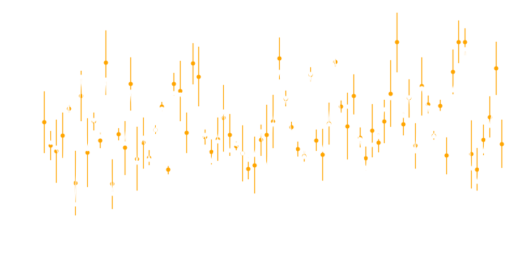 Figure 2. Example of a stochastic process with measurement noise. The observed values have heteroskedastic noise (orange dots with errorbars). The actual stochastic process is driven by the noise-free ("true") values in white, connected by white lines.