Start
Research
Publications
Statistics playground
Teaching
CV
Contact
Standard textbook methods for fitting data always assume that the "x axis" has no measurement errors (e.g. least-squares fitting). Unfortunately, this is not always true in astrophysics (e.g. consider black-hole-galaxy scaling relations). If this effect is not accounted for, the resulting fit will be systematically wrong. Unfortunately, methods to solve such fit problems are rarely taught and most standard textbooks do not mention this at all.
Here, I only provide a brief overview and terminology, such that you have keywords to start your own research. If you have questions, you can always ask me directly.
Bisector method ... and why it is wrong
A popular method for this situation is the bisector method: First, one ignores the errors on the x axis and uses a normal least-squares fit on the y data. Second, one flips x and y, ignores the errors on y and uses a normal least-squares fit on the x data. Finally, one takes a geometric mean of both best-fit models.
Unfortunately, the bisector method is still incorrect, because it still employs least-squares fitting which itself is wrong. By taking the geometric mean of two biased least-squares fits, it often manages to "average out" its own bias to some extent, but not perfectly or reliably so.
Deming regression
The correct way of fitting a straight line (y=a+bx) to data with errors on x and y is Deming regression. The trick here is to introduce "true" data x and y, for which the straight-line model holds. One can then obtain analytic solutions for those true data, given the observed data and the fit parameters. The fit parameters themselves have an analytic solution for the intercept a, but the slope b only has an analytic solution if all x have identical errors and all y have identical errors (the errors of x and y may be different). As soon as the x and y become truly heteroskedastic (which is usually the case), the slope b requires a one-dimensional numerical optimisation. However, this is trivial, as is illustrated in Figure 1.
 Figure 1. Deming regression. Left panel: Toy data with heteroskedastic errors on both axes and best-fit straight line according to Deming regression. Right panel: Graphical optimisation of slope b with minimum at ~0.49.
NB: If all x and all y have all the same identical error, then this is referred to as "orthogonal regression".Total least-squares regression
Total regression is the generalisation of the one-dimensional case of Deming regression to higher dimensions. For instances, the task of estimating the Gaia instrument model for low-resolution BP/RP spectra can be cast as a total-regression problem, where the Gaia instrument has linear response ("instrument matrix") and needs to be calibrated using a set of standard stars that have one the one hand noisy BP/RP spectra and on the other hand noisy ground-based reference spectra.
Total regression also requires to introduce "true" values, for which an analytic solution can be found. If all x and all y have identical errors (i.e. multivariate case of "orthogonal regression") this is called Total Least-Squares (TLS) regression and has a one-shot analytic solution using singlar-value decomposition. However, as soon as the data have heteroskedastic measurement errors, numerical solutions are required.
The Bayesian way
Both, Deming regression and total least-squares regression have solutions that are conditional on estimates of "true" data. More importantly, both methods are limited to fitting straight lines (in 1D or higher dimensions). There is a Bayesian approach that is far more general (yet, also computationally more expensive).
The key idea is to also introduce "true" data through marginalisation instead of optimisation as above. This may lead to high-dimensional integration, which may be hard to do numerically. Yet, in certain situations, the marginalisation integrals exist analytically.
Application: True fractions of QSOs and galaxies in Gaia DR2 sample
As a specific case of total regression, we estimated the true fractions of QSOs and galaxies in the Gaia DR2 sample (see Bailer-Jones et al. (2019)). The situation here is that on the one hand, the observed class fractions are subject to misclassifications, which are described by a "confusion matrix" that itself is estimated from a test sample of sources with known classes. A simple inversion of this confusion matrix would produce biased results, because the confusion matrix itself is an estimate derived from noisy data.
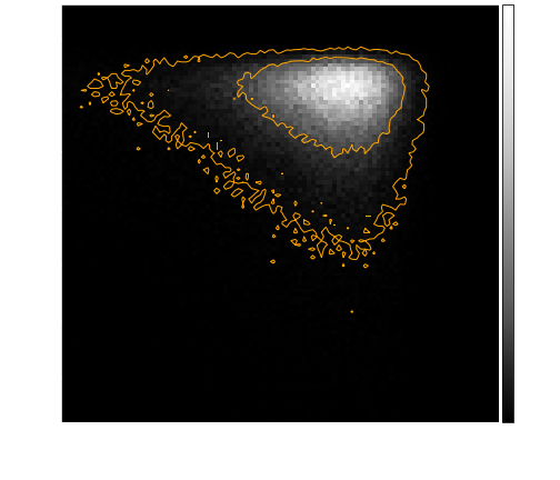 Figure 2. MCMC samples of true fractions of QSOs and galaxies in Gaia DR2 sample. Orange contours indicate confidence levels of 68.3% and 95.5%.