We're assuming here that they differ by more than their combined uncertainties. (Remember these are pseudo-Gaussian 1-sigma confidence intervals, so we do expect them to differ by more than this for 1/3 of the sources.) There are many reasons why they could differ, as discussed in the paper. For example, if the parallax SNR is low, both distance estimates will be dominated by the priors, and the priors are different. Then you probably want to use the photogeometric rather than the geometric distance (unless there is also an issue with the photometry). There are other cases where you probably want to use the geometric rather than the photogeometric distance: (1) If the source is very faint, the Gaia BP flux is often underestimated and so the source redder than reported, meaning the QG prior may be inappropriate; (2) The source may be in a crowded region, in which case the BP/RP spectrum may be blended and the colours incorrect.
No. In the limit of infinite parallax SNR, the geometric distance will converge on the reciprocal of (parallax + zeropoint). But what is a "high enough" parallax SNR for this still to be valid? There is no sharp cut-off. The whole point of doing a proper inference of distance is that we get a gradual transition from data-dominated to prior-dominated. The most valuable domain of our catalogue is probably in that transition region, which is a large fraction of the Gaia sources. But even when parallax SNR is high, there is no reason not to use the geometric distances; and they also provide sensibly-propagated distance uncertainties. Our distances also incorporate the recommended parallax zeropoint correction, which is not negligible even for nearby stars (see the question on the comparison to GCNS).
Yes. This is why our estimates are quantiles of the posterior, rather than the mean or mode. See section 1, bullet 5 of the paper.
Yes, but the convergence noise is generally much smaller (<10%) than the quoted 68% confidence interval. See the question on changing the parallax zeropoint for more details.
Maybe. The GeDR3 parallaxes are inferred assuming the source is single, and our distance estimates assume this too. If the parallax is corrupted by any binarity, our distance estimates will be too. Whether this is the case depends on whether we talking about an unresolved or a resolved binary. If resolved, and the period is much longer than the GeDR3 baseline (3 years), then the parallaxes might be okay. They might also be okay if the sources are unresolved and the period is much shorter than the GeDR3 baseline.
The GCNS aims to identify all GeDR3 sources that lie within 100pc by identifying sources with spurious parallax solutions. (The full catalogue includes all GeDR3 sources with parallax > 8 mas; 331 312 sources.) Most sources within 100pc have high signal-to-noise ratio (SNR) parallaxes, and so the distance estimates are very similar to ours in most cases. Both our and the GCNS estimates are the median of Bayesian posteriors. However, there are two potentially important differences. First, the GCNS uses (more or less) a uniform space density prior, P(r) ~ r^2 (their Figure 4). For our estimates we use a generalized gamma distribution distribution, although this is close to P(r) ~ r^2 at these short distances. Second, GCNS does not correct for the parallax zeropoint offset. For our estimates we use the functional fit published in the GeDR3 release paper.
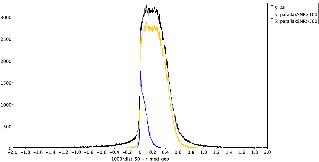
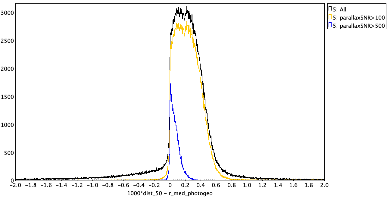
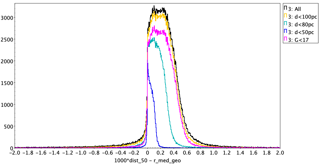
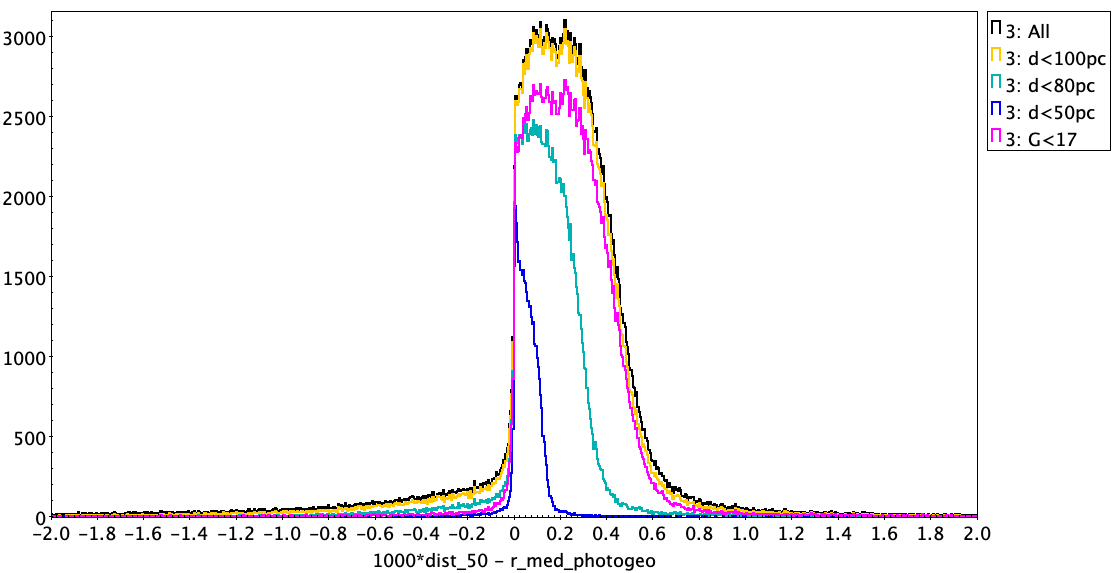
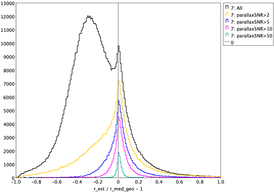
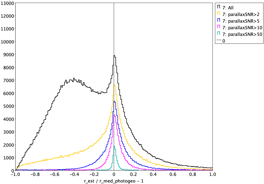
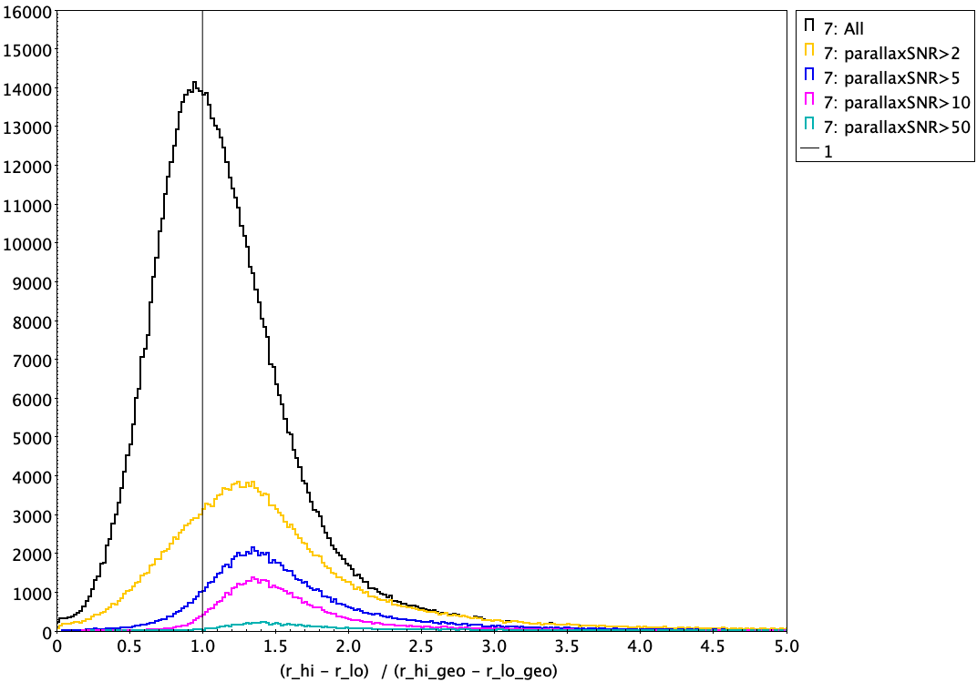
The top two plots below compare the GCNS distances with our geometric and photogeometric distances, for all common sources (323 431 sources; black line), as well as those subsets with parallax SNR greater than 100 (249 380 sources; orange) and 500 (114 394 sources; blue). The vertical axis is counts per bin. We see a clear systematic offset, in the sense that on avergae the GCNS distances are larger by 0.22 pc relative to geometric and 0.21 pc relative to photogeometric (median differences). We see a slight dependence on the parallax SNR, suggesting the difference could be due in part to the different priors. But this only has an impact at very high parallax SNR, so this is unlikely to be the dominant cause. The bottom two plots below show the histograms for just those sources within 100, 80, and 50 pc (in all distance estimates) as well as those for G<17. This shows that the systematic is not due to spuriously distant stars in the GCNS beyond 100 pc, nor is it limited to faint stars.
|
|
|
|
|
|
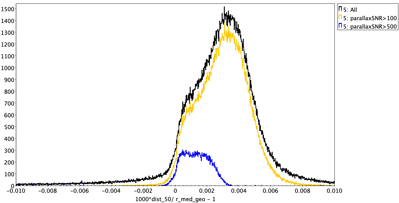
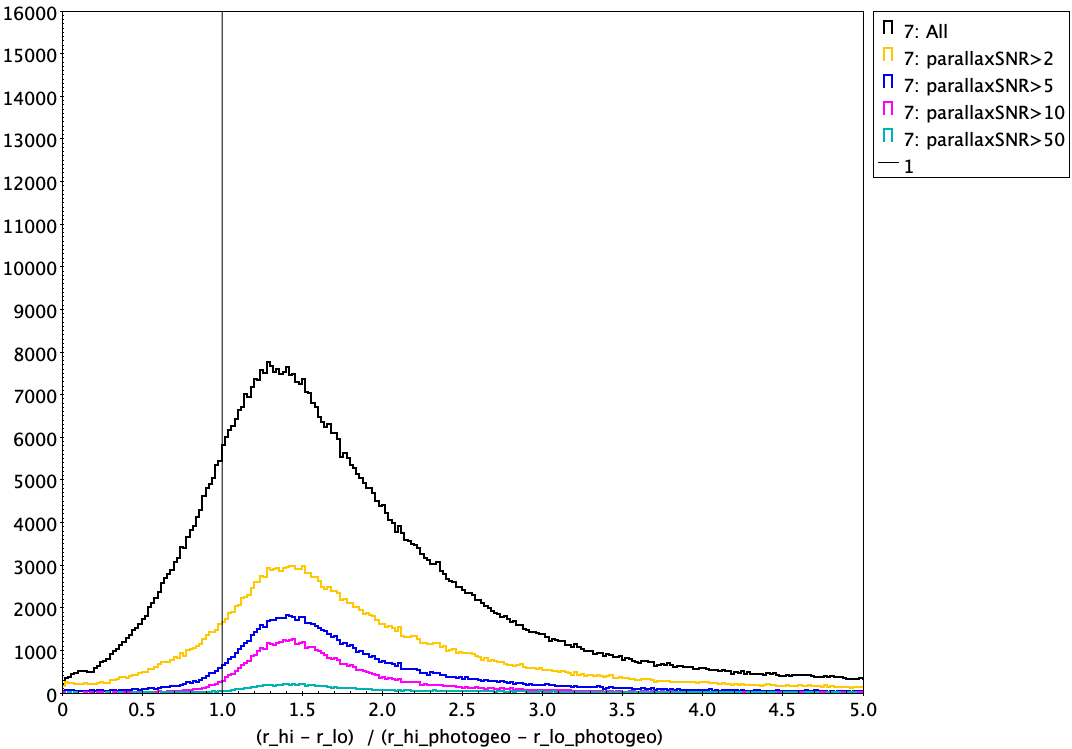
This leaves the treatment of the parallax zeropoint as a possible culprit. In the limit of the distance estimate being dominated by the data (and so the prior irrelevant), the GCNS distances will be dg = 1/w, where w is the parallax. Our distances will be db = 1/(w - wzp), where wzp is the parallax zeropint. We used the zeropoint function recommended in the GeDR3 release paper, but on average this is about -0.020 mas (note the negative sign). The ratio of these distance estimates is dg/db = 1 - wzp/w. As the median distance in the GCNS is about 80pc, or w=12.5mas, we expect dg/db = 1.0016 on average. In other words, we expect GCNS distances to be around 0.16% larger than our distances (or 0.13 pc for the average star at 80 pc) just due to the neglect of the zeropoint. This is of the order of what we actually see in the data, as is apparent from the histogram of dg/db (minus 1) shown below. For the very high parallax SNR sample the distribution is pretty much centred on 0.0016. It's not a delta function because the actual zeropoint applied depends on sky position, magnitude, and colour. For lower parallax SNR the distribution is broader and shifted to larger values, where there could also be some impact from the different choice of priors.
 |
The most obvious difference is that we use the more accurate and more precise parallaxes from GeDR3. But there are two other significant differences:
 |
 |
 |
 |
If it doesn't make a large change in the parallax, yes.
If the fractional parallax uncertainty (fpu) is small, then to a reasonable approximation the distance is r=1/w, where w is the zeropoint-corrected parallax. Suppose we want to change this parallax by dw, where dw/w << 1. From a first order Taylor expansion, dr/r = -dw/w = -r dw. (Note the sign: increasing the parallax decreases the distance.) Thus the change in distance is dr = -r^2 dw. Note that we compute a change in the distance to add to the published distances. So for a source at 2 kpc, a change in the parallax of -0.010 mas changes the distance by a fraction +0.02 (+2%), and the distance itself by +0.04 kpc.
How well does this approximation work in practice? To evaluate that we need to infer the distances from scratch using the method in the paper and the modified parallaxes. For the sake of this exercise I use much longer MCMC chains (and burnin) than I did in the paper (and published catalogue), by a factor of 100. The reason for this is that there is still some convergence noise in the published estimates due to the relatively short chains used. (This was done because of CPU limitations, impatience, and to keep the environmental impact low.) Convergence noise means if the MCMC is re-run from a different starting point, the median (or other quantile) of the chain is not identical. This noise is generally small compared to the quoted confidence intervals, but it's not zero, and it just goes to show that the confidence intervals mean something real and are not just something we are meant to quote!
Below I list three estimates of the geometric and photogeometric distances for each star: (a) the one published in the catalogue; (b) a new one using longer MCMC chains; (c) a new one using longer MCMC chains and decreasing the parallaxes by 0.014 mas (to reflect a change in the global parallax zeropoint). I show the results below for three stars with different fractional parallax uncertainties, compute dr between (c) and (b), and compare this to the approximation. All have well-behaved and well-sampled posteriors.
Columns of results (as in published catalogue; all distances in pc):
source_id,rMedGeo,rLoGeo,rHiGeo,rMedPhotogeo,rLoPhotogeo,rHiPhotogeo,flag

### hp5=10465, source_id=5891675303053080704 (fpu = 0.016)
GeDR3 catalogue:
5891675303053080704,707.516674765963,696.390096255978,717.717031977218,709.144780559287,697.88487771544,718.83098923937,10033
Original ZP:
5891675303053080704,710.490463309458,699.550572182036,721.642963524851,710.468936598579,699.550225391728,721.798957933696,10033
Modified ZP:
5891675303053080704,717.582966224147,706.431249868031,728.875073827804,717.421281502251,706.377707973145,728.845964939383,10033
dr (modified-original): geo=7.09, photogeo=6.95
Cf. the 1/w approximation from orig (dr = -r^2 dw) gives: geo=7.07, photogeo=7.07

### hp5=9479, source_id=5336389564126521728 (fpu = 0.100)
GeDR3 catalogue:
5336389564126521728,6633.12946460961,6017.6086784142,7440.78155402512,6661.19728004443,5996.31024699496,7558.429887824,10033
Original ZP:
5336389564126521728,6571.16011083943,5995.4875515791,7256.50525375428,6573.59497284227,5980.93647236675,7283.52219976453,10033
Modified ZP:
5336389564126521728,7179.65283498387,6510.46397267681,7999.94956560781,7186.29426296055,6497.1831152495,8012.09171751613,10033
dr (modified-original): geo=608.5, photogeo=612.7
Cf. the 1/w approximation from orig (dr = -r^2 dw) gives: geo=604.5, photogeo=604.9

### hp5=3573, source_id=2011892703004353792 (fpu = 0.038)
GeDR3 catalogue:
2011892703004353792,3175.53007576317,3049.06175030335,3319.56370681402,3150.63600735069,3047.60946200217,3282.08871596249,10033
Original ZP:
2011892703004353792,3173.69141875246,3052.23213118636,3304.00507726317,3168.83416124009,3048.08431747596,3298.17233328747,10033
Modified ZP:
2011892703004353792,3320.3370180146,3187.47844523341,3465.24831082359,3314.18550692321,3183.04007549041,3457.49032975933,10033
dr (modified-original): geo=146.6, photogeo=145.4.
Cf. the 1/w approximation from orig (dr = -r^2 dw) gives: geo=141.0, photogeo=153.8
Conclusion: If the fractional change in the parallax is not too large, say less than 10%, then the above approximation to modify the distance is okay. It can be applied to both the estimate and the confidence bounds for both geometric and photogeometric distances. Of course, there may be some sources with less smooth photogeometric priors (e.g. if they have extreme colours or sit in relatively empty parts of the CQD) such that this approximation is poor.
I did not save them, as they take up too much space. But I am happy to compute new chains (with more samples and burnin) for a subset of stars. Get in touch via email.