• View
• Edit
• History
• Print

Fringetracking

Questions addressed: How well did the fringe tracking work? How good is my Signal-to-Noise? Which options should I use for weak sources?

Exercise (based on instructions by WJ on 11/7/08):

• read in some .fringes.fits data, e.g. gd = oirgetdata('cal.fringes.fits')
  • plot,fringes.opd[1] gives the delay line OPD of each frame. It is changed only when needed, i.e. when the OPD shift gets too large for the internal MIDI piezos to correct for it. You can see that during frames [80:520] the OPD is offset by a large value (to -4mm) in order to measure the noise.
  • plot,fringes[0:2000].localopd[0] shows you the instrumental OPD variation, i.e. for off-set tracking you will see a zig-zag pattern from 0 to -8.5\cdot10^{-5} every 40 frames.
  • The following series of commands will give you a plot of the instrumental OPD over the fringe pattern:

    window,0,ysize=171,xsize=800
    tvscl,transpose(fringes[1000:1800,*].data1)
    plot,fringes[1000:1800].localopd[0],xstyle=4,ystyle=4,xmargin=[0,0],/noerase

• opd=oirgetopd('cal.fringes.fits') will give you a float array of the tracking OPD in microns

• In the next step of midipipe the instrumental delay is removed and the file is output as an .insopd.fits file. This is now (pseudo)complex data. One can visualise it as follows:

  rotdata = oirgetdata('cal.insopd.fits')
    complexdata = pseudocomplex(rotdata.data1)
    tvscl,abs(complexdata[indgen(1000)+1000,*])

• read in some .groupdelay.fits data, e.g. gd = oirgetdata('cal.groupdelay.fits'). This data is again pseudocomplex, so you need to do gd2 = pseudocomplex(gd.data1) to make it IDL-complex data. Then call tvscl,abs(gd2cal[1024:2048,*]) to see the delay function of the frames 1024 to 2048.

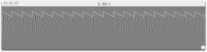
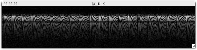
Another way to read in groupdelay.fits data is to use 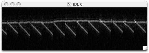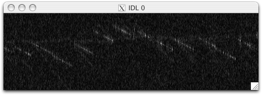c=midigetcomplex('/tmp/2010-05-27/s7','groupdelay'). This returns directly IDL COMPLEX data which are the direct Fourier transform of each frame (from frequency to delay space). This data can be displayed (as below) using tvscl,abs(c[1000+indgen(1000),*]) or tvscl,rebin(abs(cs),1000,512) or tv,0.01*rebin(abs(cs),1000,512)

The above plots have been created with the command

window,0,xsize=500,ysize=150
tvscl,abs(gd2cal[1024:1548,160:310])

The upper plot is the calibrator star, the lower one a faint science source: In the calibrator star there are only two lines: a more or less straight one that corresponds to the correct OPD and a sawtooth one that moves twice as fast as the instrumental delay. In the science image there are three lines: A very faint more or less straight line that is again the correct OPD and two sawtooth lines. The one with the greater angle towards the straight one is the one that corresponds to twice the intrumental delay. The one in between that is the brightest one here, corresponds to the sky signal. This signal is uncorrelated and thus by rotating it by -d_{ins} (i.e. what oirRotateInsOpd does) it appears as a signal that varies with d_{ins}. The signal that moves with twice the instrumental delay is also the true signal that has been modulated with the d_{ins}. The reason for this lies in the details of beam combination in MIDI: It produces a groupdelay peak at positive and one at negative delays. When subtracting (derotating) the instrumental OPD from both, one becomes a straight line and the other one is seen as a peak that varies twice as fast as the original modulation. A few more technical details on this can be found in Walter's description of oirGroupDelay.

While the data has already been smoothed at this step in midipipe (gsmooth has been applied), the data that is read in with oirgetdata (see above) is not yet smoothed. To do this by hand, call 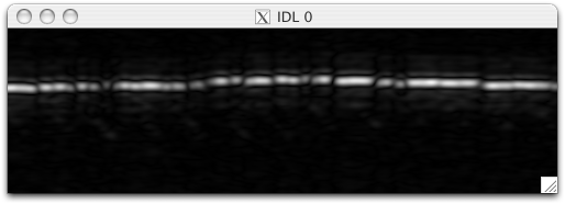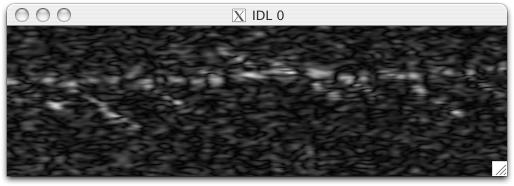gd2cals=csmooth2(gd2cal,4) and then display the data: tv,abs(gd2cals[1024:2048,*])*0.001

The top image is the smoothed calibrator, the lower one the smoothed science source. The value for smoothing (gsmooth) was 4 (default). One can see that the wrong OPD information has been very nicely removed from the calibrator star. But in the science source the sky signal dominates and therefore some sky signal remains that might distract the fringe tracking algorithm.

Of course one can try a larger value of gsmooth, e.g. gsmooth = 20: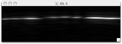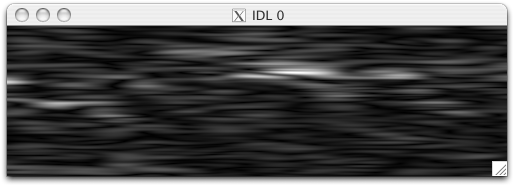

A larger value smoothes over more frames, i.e. over more time. So it is only appropriate when weather conditions were good so that the frames that are smoothed together are within a coherence time. Here, one can see that the larger value of gsmooth has not affected the calibrator data too much, but in the science source almost nothing is left.

But there is a better way of getting rid of the sky background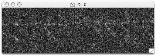: dave. In order to use this function in the data reduction one has to select off-set tracking already during the observations. For weak sources, one should therefore always use off-set tracking. If dave is set (/dave in midipipe), then during oirFormFringes all pixels of each frame are averaged and subtracted from that frame. This suppresses the sky background but it also lowers the correlated flux if the fringe was scanned over the zero OPD position as both the sky and the source signal are then mixed at the zero position. If dave is set, the autoflagger flags all points where the tracking is close to zero OPD.

The dave-treated science data then looks like this:

After smoothing with the default value (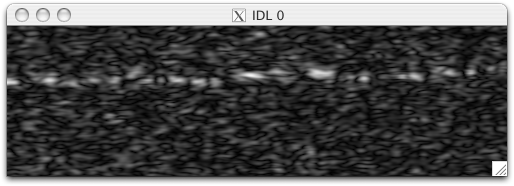gsmooth = 4) one gets:

For 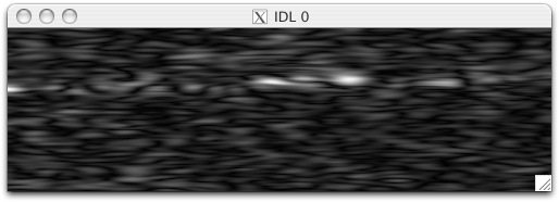gsmooth = 10 it looks like this:

And for 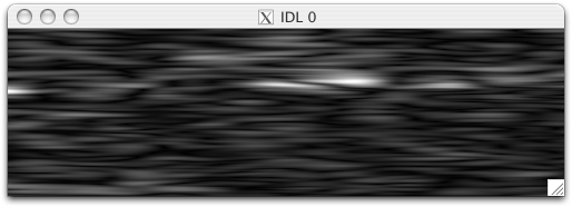gsmooth = 20 it looks like this:

From this exercise we see that the Signal to Noise ratio for this particular science observation was not very good: There are many places where the signal is not visible over the background.

Next, we can plot the delay that the fringe tracker has found from the above result:

d = oirgetdelay('tag.groupdelay.fits')
dd=reform(d.delay)
dd=dd-median(dd)

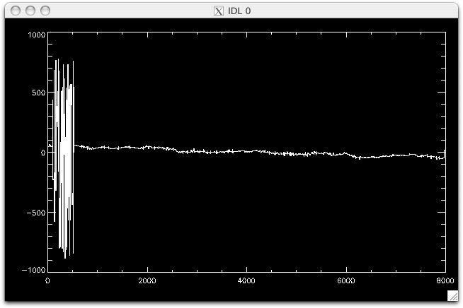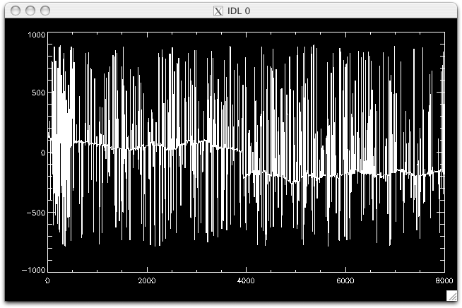For this, the fringe tracker picks the brightest spot. One can clearly see the difference between the science and the calibrator source: Whereas the delay could be easily and steadily determined for the calibrator source (upper image), the delay plot of the weak science source has many jumps, indicating that the delay could not be determined reliably for every frame.

We can also overplot the delay the fringe tracker found over the delay function to make clear when and why the fringe tracker could not find the correct groupdelay: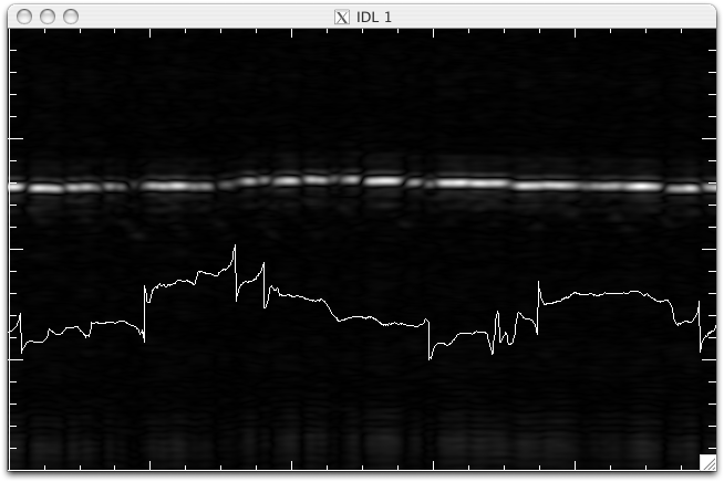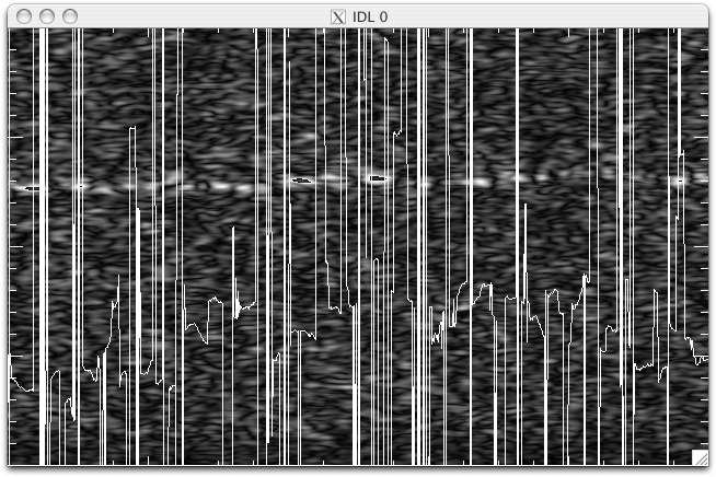

The above was produced using

d=oirgetdelay('sci.groupdelay.fits')
gd1=oirgetdata('sci.groupdelay.fits')
gd2=pseudocomplex(gd1.data1)
gd2s=csmooth2(gd2,5)
tv,0.01*rebin(abs(gd2s[1000+indgen(1000),*]),1000,512)
plot,-d.delay,xr=[1000,2000],/noerase,charsize=0.01,yr=[-100,100]

Here we only plotted a 1000 pixel wide segment of the fringe track. You can see again that, for the science source (lower image), the signal/noise is bad in many frames (i.e. columns) and the OPD position that the fringe tracker returned has many jumps or spikes. For the calibrator (upper image) on the other hand the found OPD position is in most parts a smooth line. The y range of both plots is [-100 µm, +100 µm].